Data-driven discovery of dynamical systems

The problem

A large chunk of applied mathematics aims to understand dynamical systems and to characterize their behavior.

But what happens if you have a physical system for which you don’t know the governing equations?

You might suspect that there is a set of differential equations pulling the strings, but maybe you are unable or unwilling to derive them analytically.

If you can get your hands on measurements of the system, then you may be able to use a data-driven approach.

A solution

One recently developed method for nonlinear model discovery is the Sparse Identification of Nonlinear Dynamical systems (SINDy).

How it works

The main idea is that the right-hand sides of many dynamical systems of interest do not include many terms, implying that they are sparse with respect to an appropriately chosen basis.

Suppose we have measurements $x(t)$ of a physical system over time. SINDy seeks to represent the time evolution of $x(t)$ in terms of a nonlinear function $f$, defining a dynamical system model for $x(t)$: $$ \frac{d}{dt}x(t) = f(x(t)). $$

The vector $x(t)=[x_1(t), x_2(t), \dots x_n(t)]^\top$ gives the state of the physical system at time $t$. The function $f(x(t))$ constrains how the system evolves in time.

In many problems of interest, $f$ turns out to be sparse in the set of possible basis functions. For example, the function

$$ \frac{d}{dt}x = f(x) = \begin{pmatrix} f_1(x) \\ f_2(x) \end{pmatrix} = \begin{pmatrix}1 - x_1 + 3x_1x_2 \\ x_2^2 - 5x_1^3 \end{pmatrix} $$

is sparse with respect to the set of polynomials in two variables in the sense that just a few of the infinite number of polynomial terms are present on the right-hand side of the equation. So if we pick an appropriate basis ${\theta_1, \theta_2, \dots, \theta_k}$ then it is often possible to express each component of $f$ (note that $f$ is often vector-valued) as

$$ f_i(x) \approx \xi_1 \theta_1(x) + \xi_2\theta_2(x) + \dots \xi_k\theta_k(x) $$

with most coefficients $\xi_j$ being zero. SINDy leverages sparse regression to identify the active terms in the dynamics (the nonzero coefficients $\xi_j$).

Mathematical formulation

To apply SINDy one needs a set of measurement data collected at times $t_1, t_2, \dots, t_n$, and the time derivatives of these measurements (either measured directly or numerically approximated). These data are aggregated into the matrices $X$ and $\dot X$, respectively

$$ X = \begin{bmatrix} x_1(t_1) & x_2(t_1) & \dots & x_n(t_1) \\
x_1(t_2) & x_2(t_2) & \dots & x_n(t_2) \\
\vdots & \vdots & & \vdots \\ x_1(t_m) & x_2(t_m) & \dots & x_n(t_m) \end{bmatrix}, $$ $$ \dot{X} = \begin{bmatrix} \dot{x_1}(t_1) & \dot{x_2}(t_1) & \dots & \dot{x_n}(t_1) \\
\dot{x_1}(t_2) & \dot{x_2}(t_2) & \dots & \dot{x_n}(t_2) \\
\vdots & \vdots & & \vdots \\
\dot{x_1}(t_m) & \dot{x_2}(t_m) & \dots & \dot{x_n}(t_m) \end{bmatrix}. $$

Next, one forms a library matrix $\Theta(X)$ whose columns consist of a chosen set of basis functions applied to the data

$$ \Theta(X) = \begin{bmatrix} \mid & \mid & & \mid \\
\theta_1(X) & \theta_2(X) & \dots & \theta_\ell(X) \\
\mid & \mid & & \mid \end{bmatrix}. $$

We seek a set of sparse coefficient vectors (collected into a matrix)

$$ \Xi = \begin{bmatrix} \mid & \mid & & \mid \\
\xi_1 & \xi_2 & \dots & \xi_n \\
\mid & \mid & & \mid \end{bmatrix}. $$

The vector $\xi_i$ gives the coefficients for a linear combination of basis functions $\theta_1(x), \theta_2(x), \dots, \theta_\ell(x)$ representing $f_i$, the $i$th component function of $f$, i.e. $f_i(x) \approx \Theta\left(x^\top\right) \xi_i$ (note that the preceding equation should be interpreted as a symbolic expression).

Finally, we are ready to write down the approximation problem underlying SINDy:

$$ \dot X \approx \Theta(X)\Xi. $$

A sparse regression algorithm is then employed to solve the related minimization problem

$$ \min_{\Xi} \frac{1}{2}\|\dot{X} - \Theta(X)\Xi\|_F^2 + R(\Xi), $$ where $R$ is a sparsity-promoting regularization function such as $\|\cdot\|_1$.

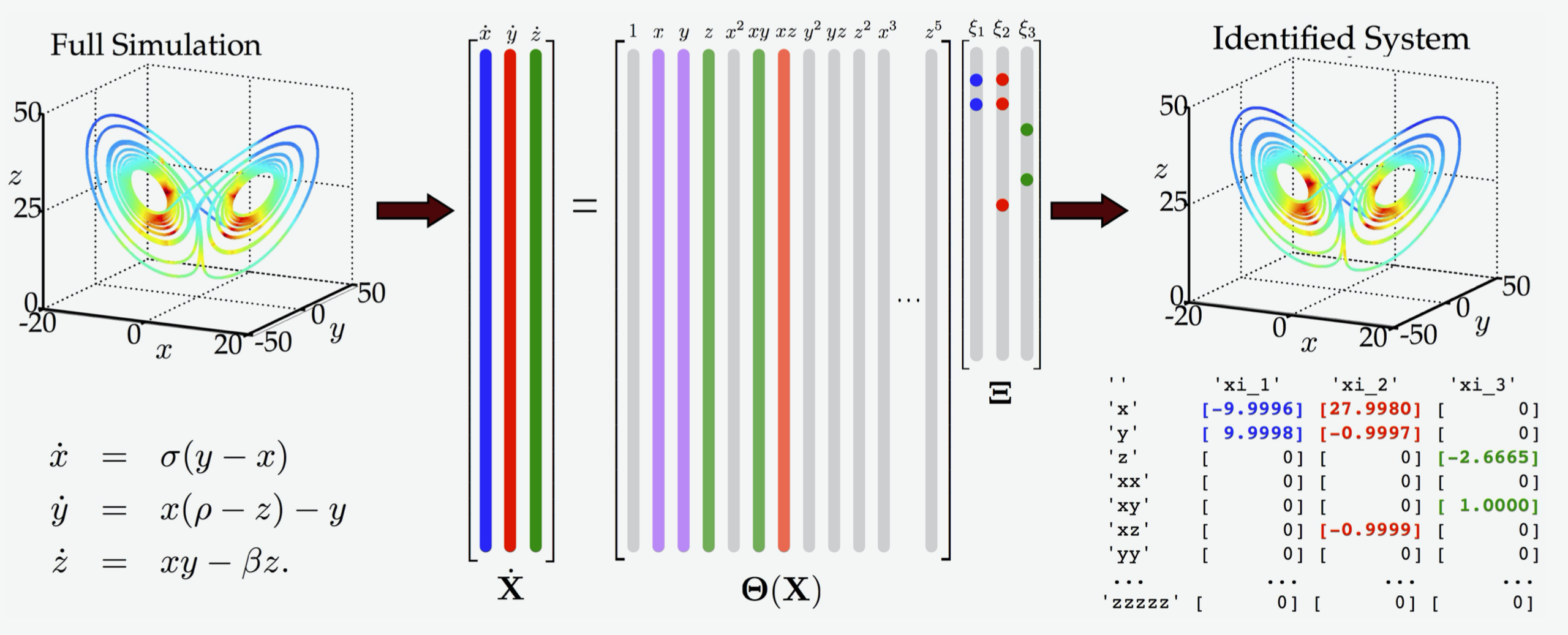
The following image shows an overview of the SINDy method applied to the Lorenz equations.

Image summary of the SINDy method

Resources